Catalog of OMA Tools
We have developed several computational tools to facilitate user-side analyses using the OMA database. These tools are implemented either online, as software, or as interactive visualizations of the data.
Online Tools
Fast Mapping
The ever accelerating pace of genomic sequencing is such that OMA can only focus on a subset of all public genomes available. Many will remain absent from orthology databases such as OMA. Thus, there is an interest in efficiently transferring knowledge from orthology databases to genomes provided by the user. In (Altenhoff et al. 2018), we introduced GO function prediction tool based on fast mapping to the closest sequence. In the last release, we have improved the performance of the fast sequence mapper, which mainly relies on a k-mer index. On the current OMA server, the mapper can process approximately 200 sequences per second, meaning that a typical animal genome can be processed in less than 2 minutes. It remains possible to infer GO annotations based on the closest sequence. Alternatively, users can retrieve the closest match for all input sequences—either across all of OMA, or in a target genome.

OMA-MO: Find model organism
OMAMO is a web tool that allows the user to find the best simple model organism for a biological process of interest. The set of species consists 50 less complex organisms including bacteria, unicellular eukaryotes and fungi.
OMArk: Assess proteome quality
OMArk is a software to assess the quality of gene repertoire annotated from a genomic sequence - also called proteome. It relies on comparisons to the predicted ancestral gene repertoire of the target species and to the extant gene repertoire of close species to:
- Estimate the completeness of the gene-repertoire by comparison to conserved orthologous groups.
- Estimate the proportion of accurate and erroneous gene models in the proteome.
- Detect possible contamination from other species in the proteome.
Phylogenetic Marker Gene Export
To infer a phylogenetic species tree, it is first necessary to identify sets of orthologous genes among the genomes of interest. One of the outputs of the OMA database are OMA Groups, or sets of genes which are all orthologous to each other. Since genes in OMA Groups are related exclusively by speciation events, there is at most one sequence per species in each OMA group. In contrast to most other phylogenetic methods, OMA makes no assumption about species relationships when inferring OMA Groups. This makes OMA Groups particularly useful for phylogenetic species tree inference.
We provide a function, ‘Export marker genes’, to retrieve the most complete OMA groups for a given subset of species.
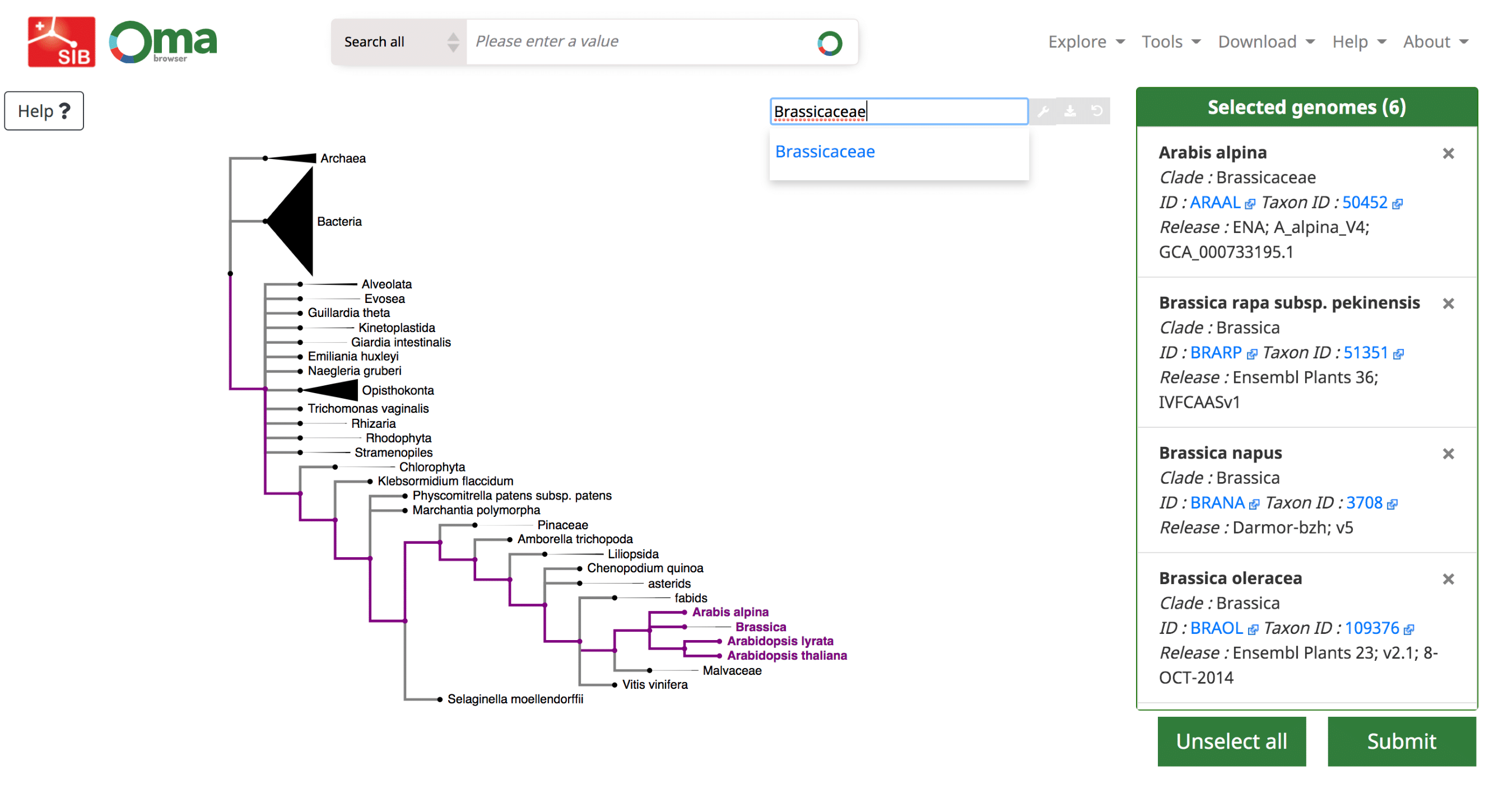
Use the Download -> Export marker genes option. This will open a page which allows the user to select species. Species can be searched by name or clade. A whole clade can be selected by clicking on the node (select all species). A single species can be selected by clicking on the leaf (select species). All selected species will be displayed in the right box with additional species information (release info, taxon id, etc.).
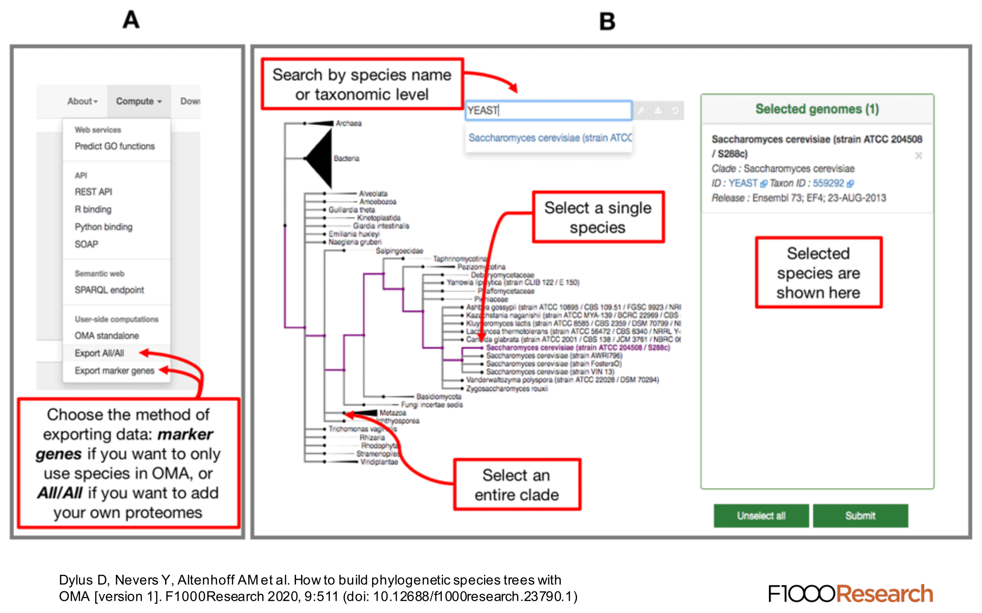
Specifying the Minimum Species Coverage and Maximum Number of Markers parameters.
After species selection, exported OGs will depend on the minimum fraction of covered species and the maximum number of markers parameters:
- Minimum species coverage: the lowest acceptable proportion of selected species that are present in any given OG in order to be exported. A more permissive (lower) minimum species coverage will result in a higher number of exported groups. Choosing this parameter depends on the number of and how closely related are the selected species. For instance, consider the Drosophila clade versus chordates clade (20 and 116 species in current release, respectively). If one selects the 20 Drosophila genomes and sets the minimum species coverage to 0.5, only OGs with at least 10 Drosophila species will be exported. In the current release, this results in 11,855 OGs which meet this criteria. If using the same 0.5 minimum species coverage for the chordates, it results in 14,357 OGs exported. On the other hand, for a 0.8 minimum species coverage, 7,886 and 6,329 OGs are exported for Drosophila and chordates clades, respectively.
- Maximum number of markers: the maximum number of OGs/marker genes to return. To consider as much information as possible in the tree inference, remove any limit by setting this parameter to -1, in which case all OGs fulfilling the minimum species coverage parameter will be returned. To speed up the tree inference, set this value to below 1000 genes.
After filling in the parameters and submitting the request, the browser will return a compressed archive (“tarball”) that contains a fasta file with unaligned sequences for each OG. Depending on the size of the request, it may take a few minutes for this operation to complete.
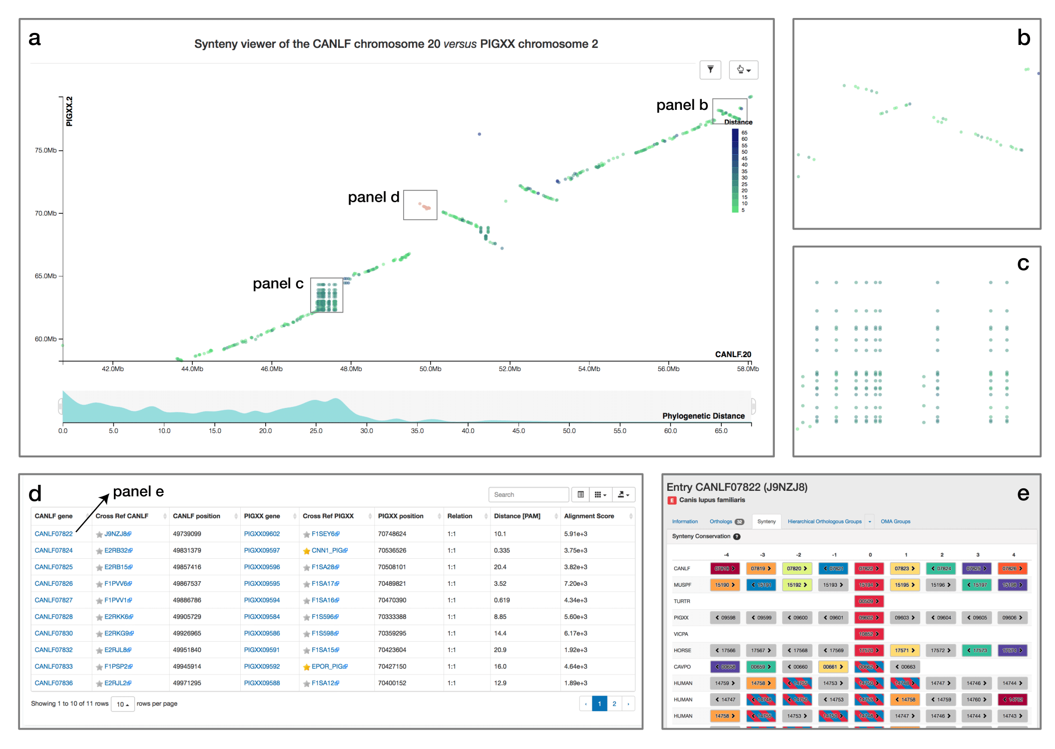
Synteny Dot Plot
When comparing two related species, the position of orthologous genes is often conserved. Positional conservation can be at the chromosomal level—e.g. when there are entire chromosomes or chromosomal segments that are orthologous between species; or it can be more local—e.g. neighboring genes in one genome are orthologous to neighboring genes in the other genome. In OMA, we refer to global synteny for the former, and local synteny for the latter (local synteny is sometimes also referred to as ‘colinerarity’). The Synteny Dot Plot complements the Local Synteny Viewer by providing a more global and interactive view of positional conservation.
If you want to visualise the synteny of a genome with another genome you need to first select a second genome in the side menu. Then, a chromosome selection widget will open and guide you to configure the viewer.
For any pair of chromosomes (in different species if we consider orthologs, or different subgenomes if we consider homoeologs), the plot draws orthologs as dots on a two-dimensional plot, where the axes are the absolute physical location of the genes along the chromosome. Diagonals in the plot can thus be interpreted as syntenic regions, and one can easily identify genomic rearrangements such as inversions, duplications, insertions, deletions and highly repetitive regions. Users can zoom on particular regions of interest and obtain more details on orthologs of interest by selecting them. Each dot is colored based on a color scale reflecting the evolutionary distance in point accepted mutation (PAM) units. Furthermore, one can filter the orthologs to a specific distance range by clicking on the filtering icon and selecting the desired range on a histogram. Other features include panning and exporting the view as a high-resolution vector graphic.
GO Functional Annotation
An important application of orthology is the ability to transfer gene function annotations from the few well-studied model organisms to the large number of poorly studied genomes. We previously described our approach to predict Gene Ontology (GO) annotations from OMA Groups (Altenhoff et al. 2015).
We now provide a feature to annotate custom protein sequences through a fast approximate search with all the sequences in OMA. The user can upload a fasta formatted file and will receive the GO annotations (GAF 2.1 format) based on the closest sequence in OMA. These results can directly be further analyzed using other tools, e.g. to perform a gene enrichment analysis.
Please see (Altenhoff et al. 2018) and (Altenhoff et al. 2015) for more information.
Orthologs between two genomes (Genome Pair View)
Use the following form to download the list of all predicted orthologs between a pair of genomes of interest. Since orthologs are sometimes 1:many or many:many relations, this download will return more orthologs than what is covered by the OMA groups. The result is returned as a tab-separated text file, each line corresponding to one orthologous relation. The columns are the two IDs, the type of orthology (1:1, 1:n, m:1 or m:n) and (if available) the OMA group containing both sequences.
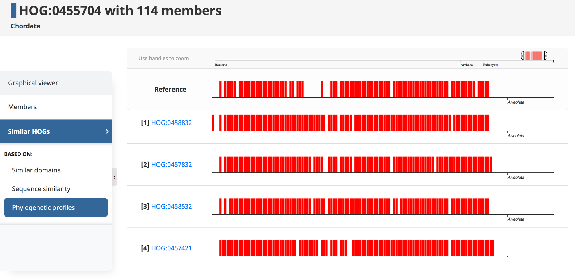
Phylogenetic profiler
Genes that are involved in the same biological processes tend to be jointly retained or lost across evolution. Thus, such co-evolution patterns can be used to infer functionally related genes—a technique known as “phylogenetic profiling.” Recently, we introduced HogProf, an algorithm to efficiently identify similar HOGs in terms of their presence or absence at each extant and ancestral node in the genome taxonomy, as well as the duplication or loss events on the branch leading to that node. This functionality has been added to the OMA browser, making it possible, starting from any HOG, to identify similar HOGs using similar phylogenetic patterns.
Under the “similar HOGs” tab, click on “phylogenetic profiles” to access the interactive visualization of the presence or absence of orthologs in different species (represented as vertical lines) in HOGs with a similar phylogenetic profile (displayed as rows).
It is important to note that the visual representation of the profile available on the web interface only shows the extant species covered by the query and returned HOGs. The actual profile similarities are calculated between the set of taxonomic nodes where ancestral presence was inferred along with extant species, as well as the set of ancestral duplications and losses shared between HOGs.
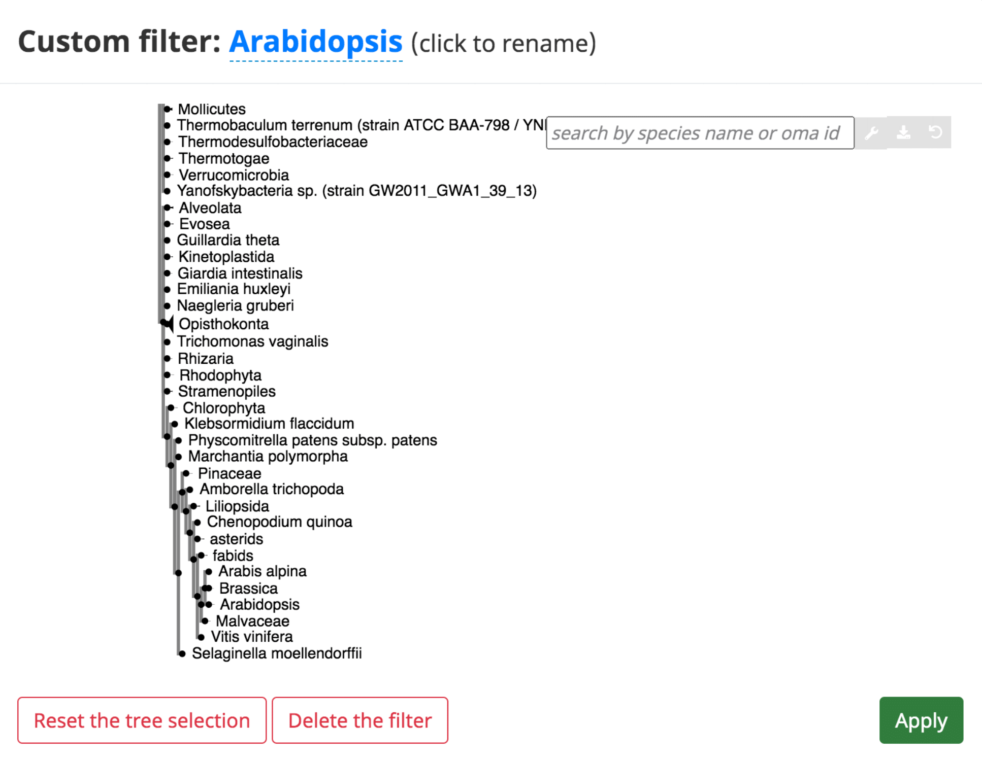
Add taxonomic filters to tables
Export the all-against-all file for a subset of species in the OMA database. Search for species using the interactive species tree or the search bar. Click on a species or node to select genomes, which are displayed on the right.
Phylogenetic Marker Gene Export
In several of the tables, it is possible to add a “custom filter” to the data. This function can be used to select only the results from a certain species or taxonomic range
Software
To enable user-side analyses we provide several softwares and libraries available for download.
OMA Standalone
OMA standalone takes as input the coding sequences of genomes or transcriptomes, in FASTA format. The recommended input type is amino acid sequences, but OMA also supports nucleotide sequences. With amino acid sequences, users can combine their own data with publicly available genomes from the OMA database, including precomputed all-against-all sequence comparisons (the first and computationally most intensive step), using the export function on the OMA website (http://omabrowser.org/export).
OMA standalone produces several types of output:
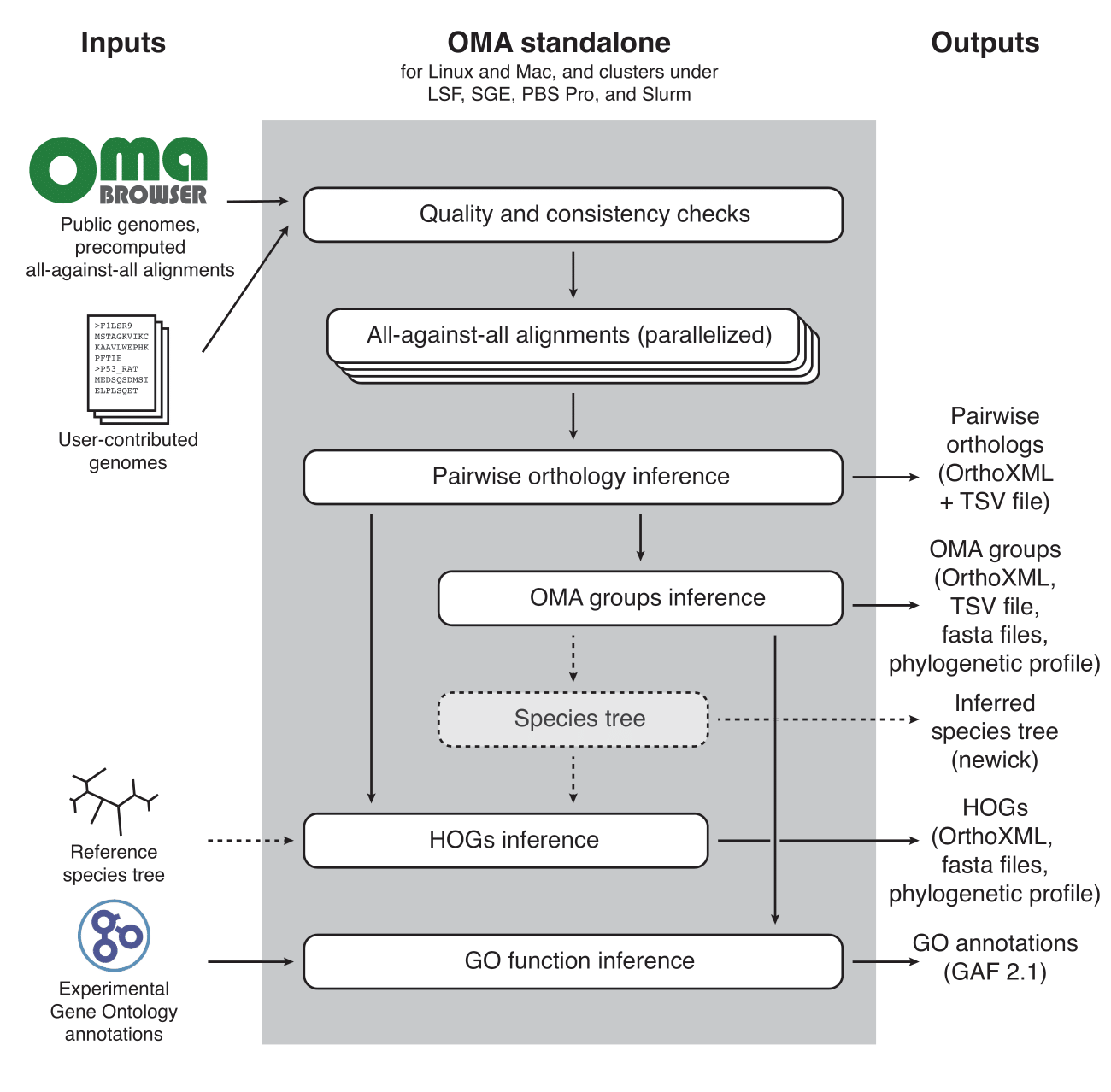 Please see (Altenhoff et al. 2019) for more information.
pyHam
We have developed a python tool called pyham (Python HOG Analysis Method), which makes it possible to extract useful information from HOGs encoded in standard OrthoXML format. It is available both as a python library and as a set of command-line scripts. Input HOGs in OrthoXML format are available from multiple bioinformatics resources, including OMA, Ensembl and HieranoidDB.
The main features of pyHam are:
- Given a clade of interest, it can extract all the relevant HOGs, each of which ideally corresponds to a distinct ancestral gene in the last common ancestor of the clade
- Given a branch on the species tree, report the HOGs that duplicated on the branch, got lost on the branch, first appeared on that branch or were simply retained
- Repeat the previous point along the entire species tree and plot an overview of the gene evolution dynamics along the tree
- Given a set of nested HOGs for a specific gene family of interest, generate a local iHam web page to visualize its evolutionary history.
- Paper: (Train et al. 2019)
- Github: https://github.com/dessimozlab/pyham
- Tutorial: https://zoo.cs.ucl.ac.uk/tutorials/tutorial_pyHam_get_started.html#object
- Blog post: http://lab.dessimoz.org/blog/2017/06/29/pyham
- Pyham website: https://lab.dessimoz.org/pyham
OMA Rest API
(See OMA Rest API under Access the Data.)
OMAdb (python package)
(See OMAdb python package under Access the Data.)
OMAdb (R package)
(See OMAdb R package under Access the Data.)
Visualization tools
iHam (Graphical Viewer)
The iHam Graphical Viewer is an interactive tool to visualize the evolutionary history of a specific gene family.
How to read the iham viewer ?
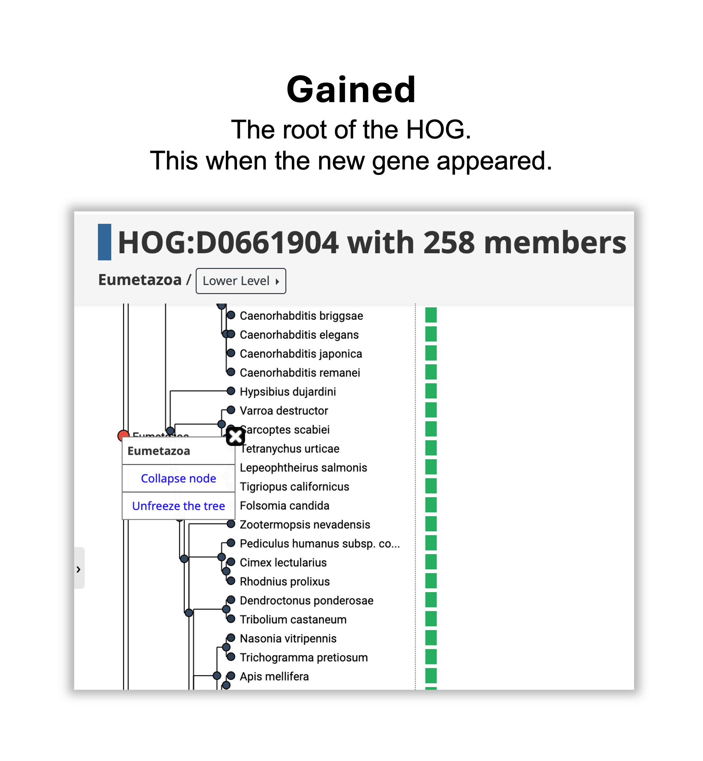
The viewer is composed of two panels: On the left is a species tree that lets the user select a node to focus on a particular taxonomic range, and on the right is a matrix that organizes extant genes according to their membership in species (rows) and HOGs (columns).
The entire composition of all the genes, visible from the root of the tree, is the gene family . The iham viewer is composed of the following elements:
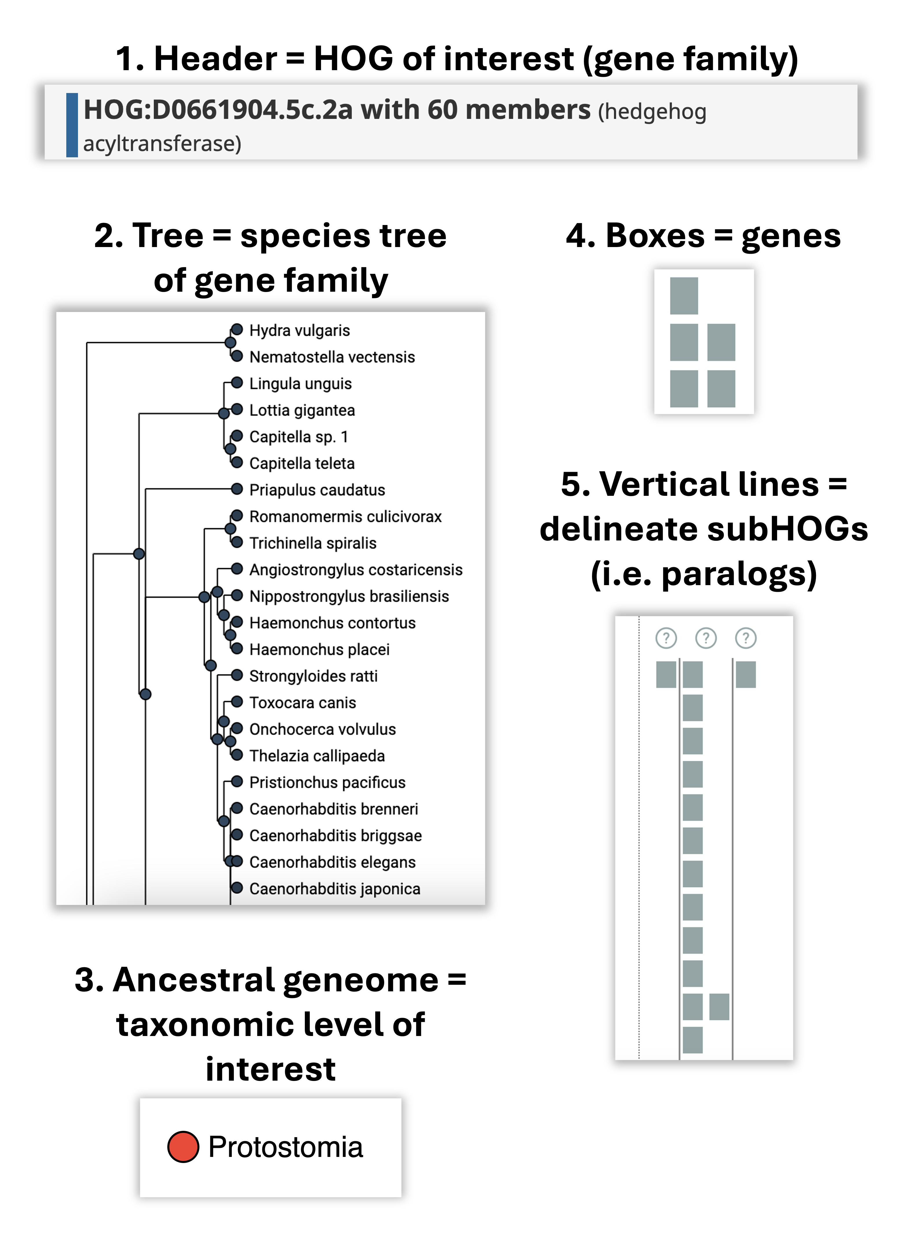
How does it all fit together? All the elements together provide a snapshot into the ancestral genome content of a gene family at a specific taxonomic level.
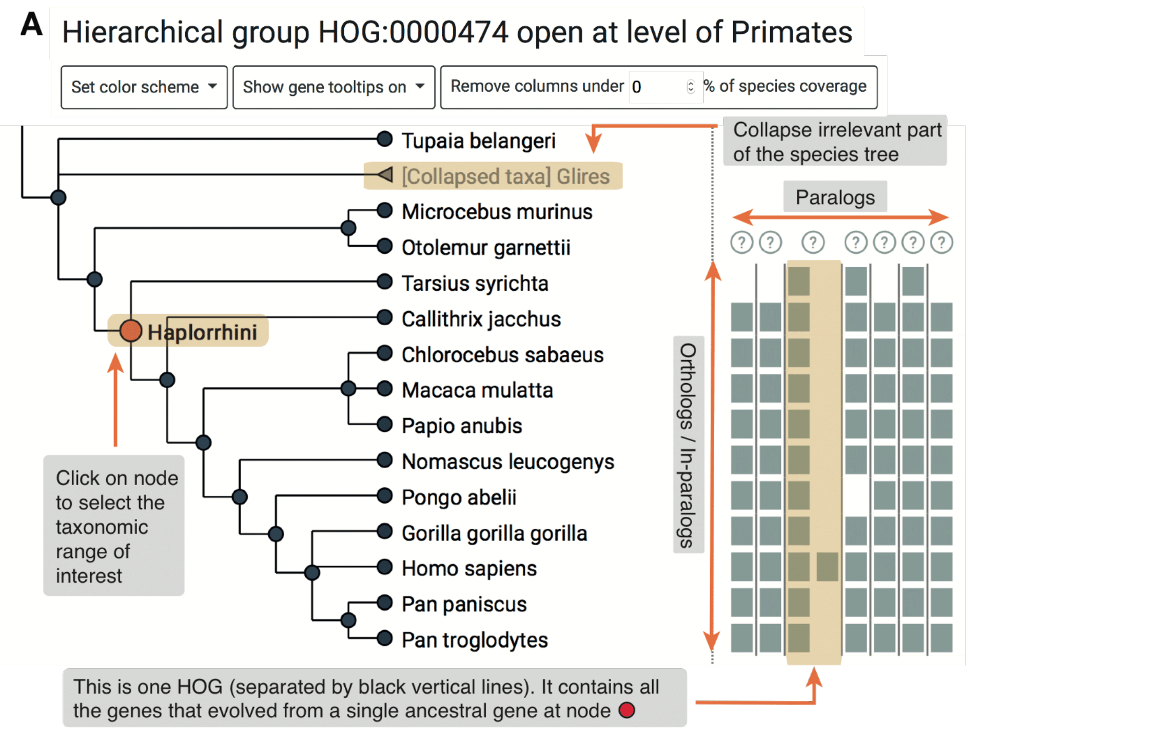
How can I infer evolutionary events?
- View an ancestral level of interest by mousing over the node in the tree. All HOGs (ancestral genes) present in that ancestral species are delineated by vertical lines.
- Mouse over subsequent internal nodes in the tree by moving closer to the leaves.
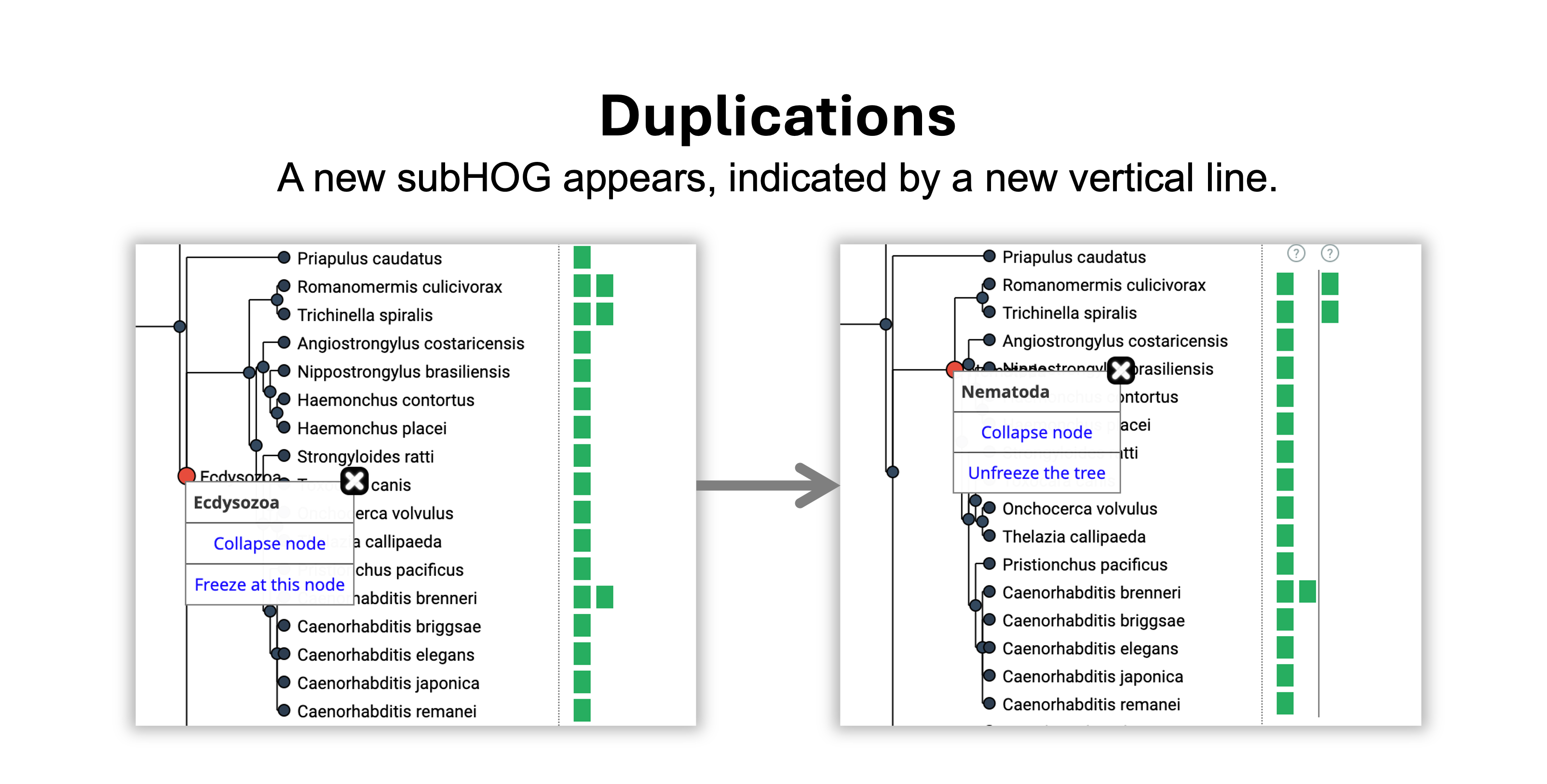
- A duplication happened on the branch leading from Ecdysozoa to Nematoda because 1 vertical line appeared.
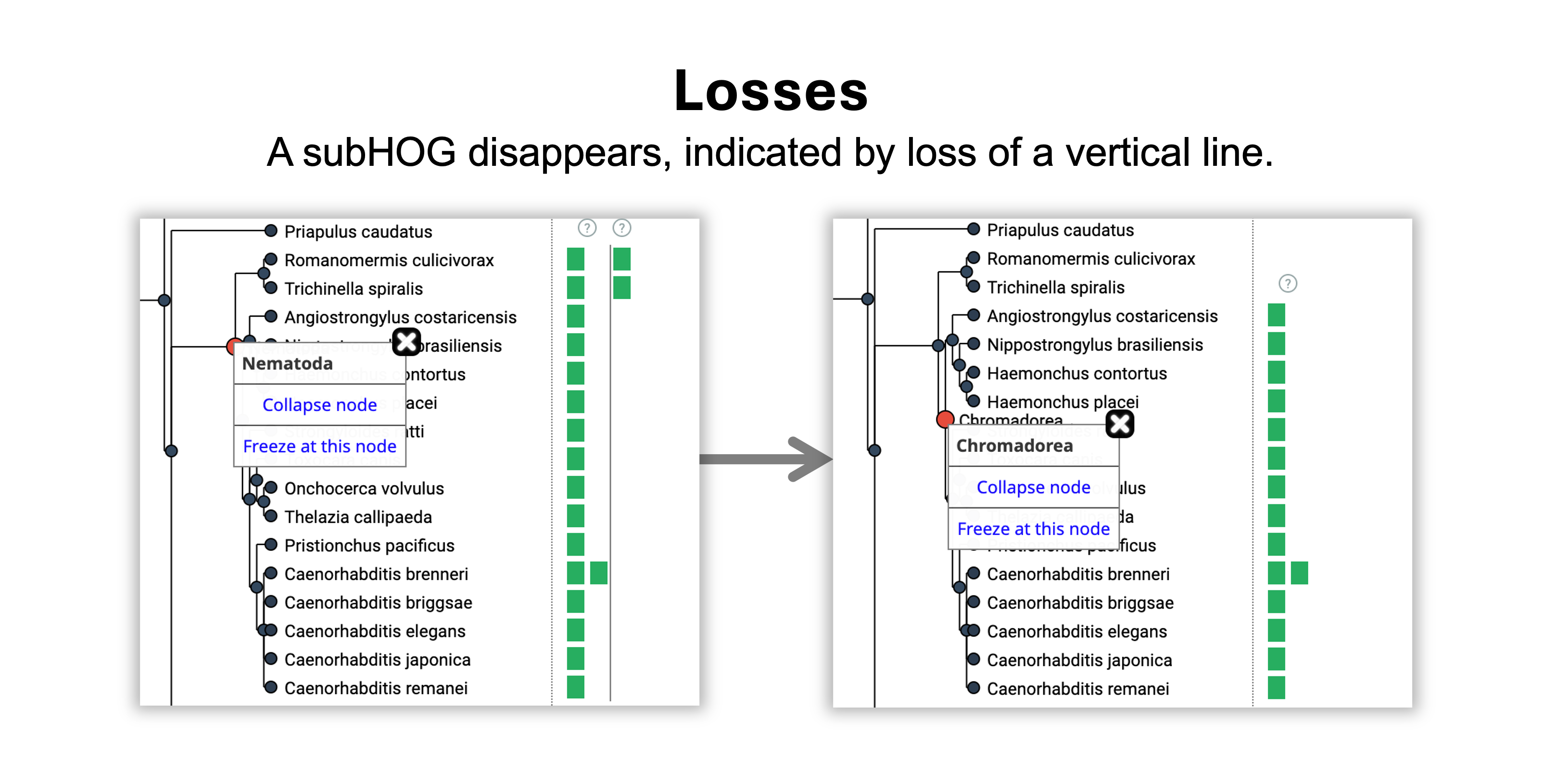
- A loss happened on the branch leading from Nematoda to Chromadorea because 1 vertical line disappeared.
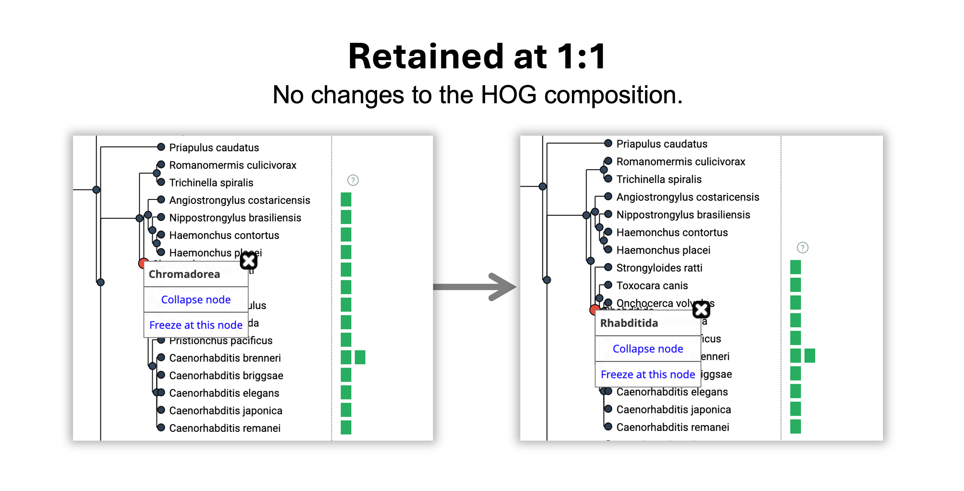
- The gene was retained without duplications or losses from the Chromadorea to the Rhabditida common ancestor.
- The gene was gained in Eumetazoa, the root level of the HOG.
Tips
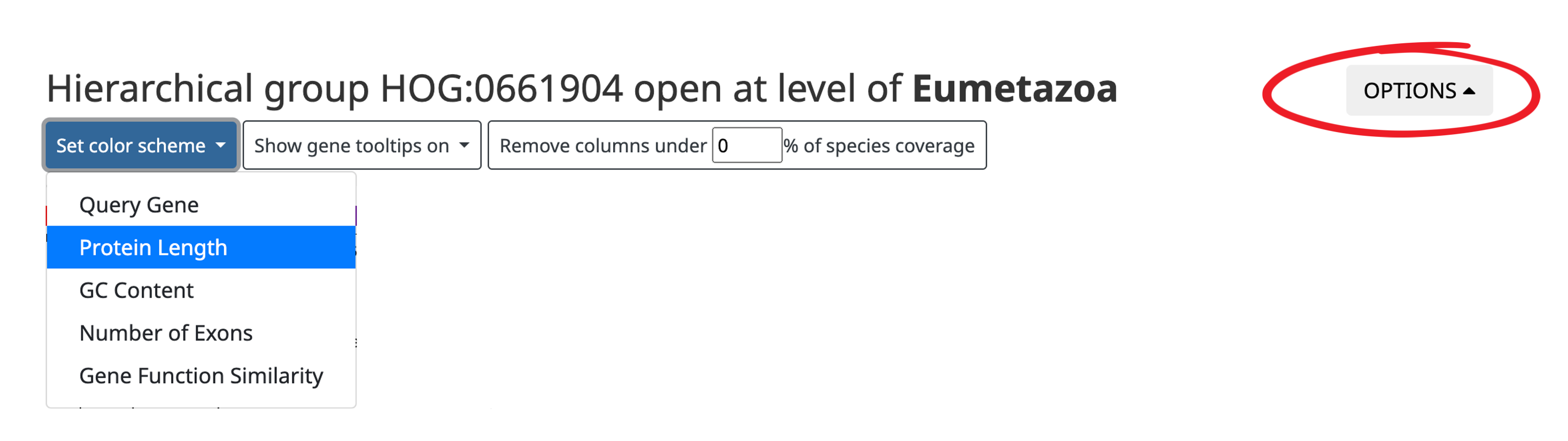
- Color genes according to protein length, GC-content, number of exons, or gene function similarity.
- If the species coverage within a HOG looks implausible, this might be due to an orthology inference error. Low-confidence HOGs can be masked based on the Completeness Score (number of species in the HOG/number of species in the clade).
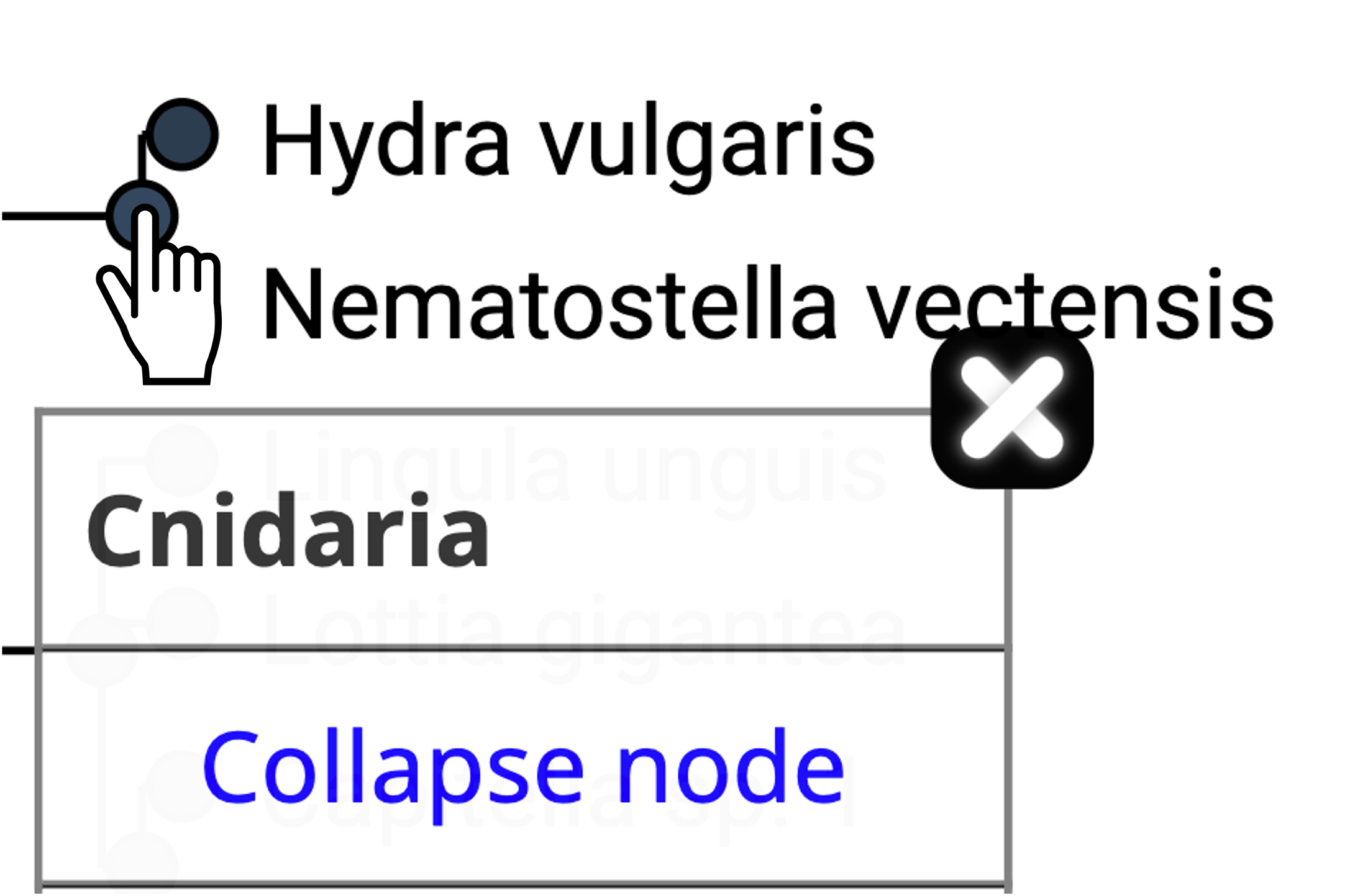
- Irrelevant species clades can be collapsed.
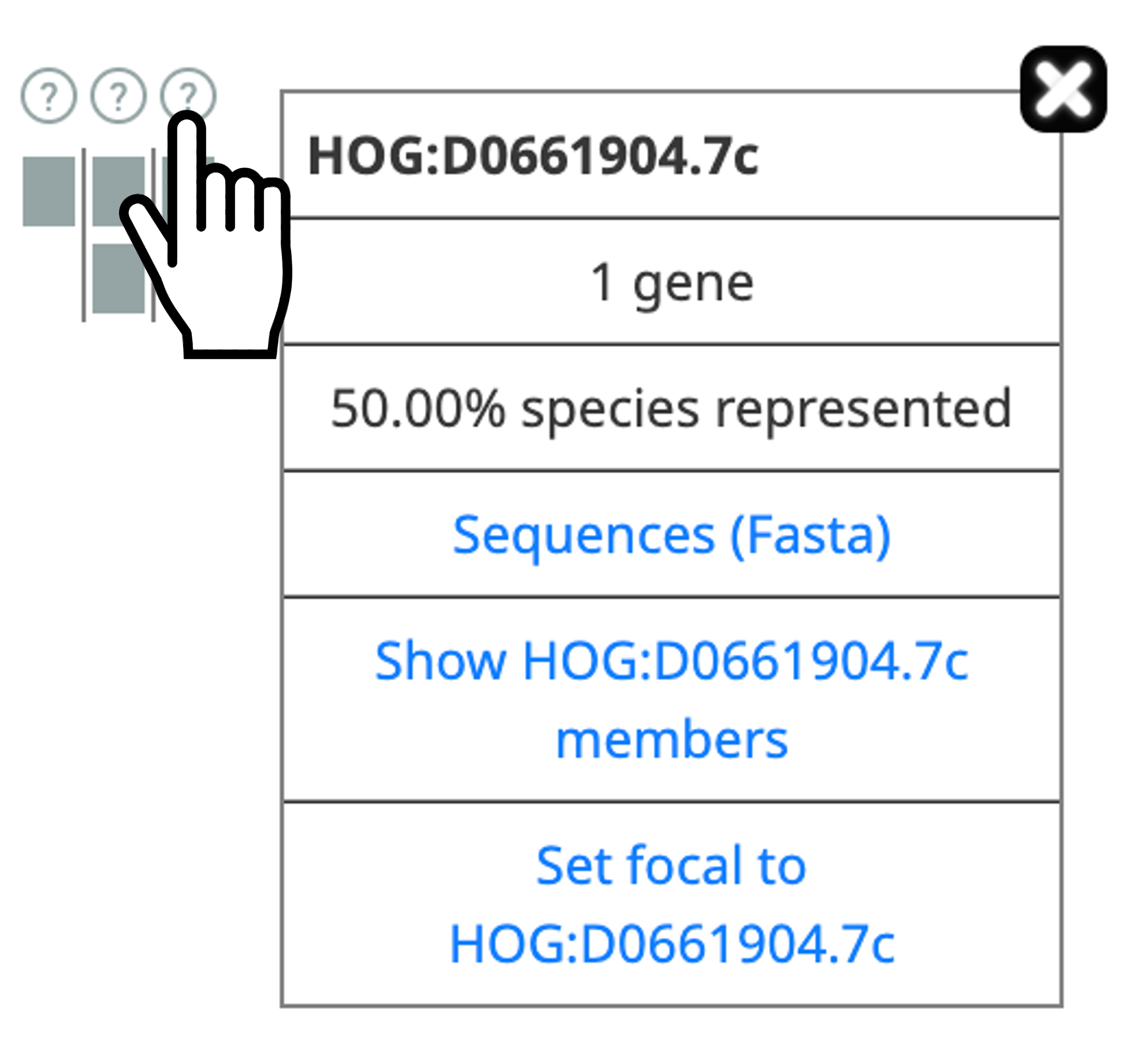
- Get more information about subHOG by clicking on (?)
- Gene more information about an extant gene by clicking on it

iHam is a reusable web widget that can be easily embedded into a website; the code is available on github. It merely requires as input HOGs in the standard OrthoXML format and the underlying species tree in newick or PhyloXML format.
Using iham ? Please cite:Clément-Marie Train et al, iHam and pyHam: visualizing and processing hierarchical orthologous groups, Bioinformatics, Volume 35, Issue 14, July 2019, Pages 2504–2506, 10.1093/bioinformatics/bty994
Species Information Viewer
In the species information viewer, you can browse through which species are in the OMA database and get more information about them.
Taxon Hierarchy View (sunburst)
The default view is the Taxon Hierarchy view. Each section in the Taxon Hierarchy View represents a clade or species at the tips of the viewer.
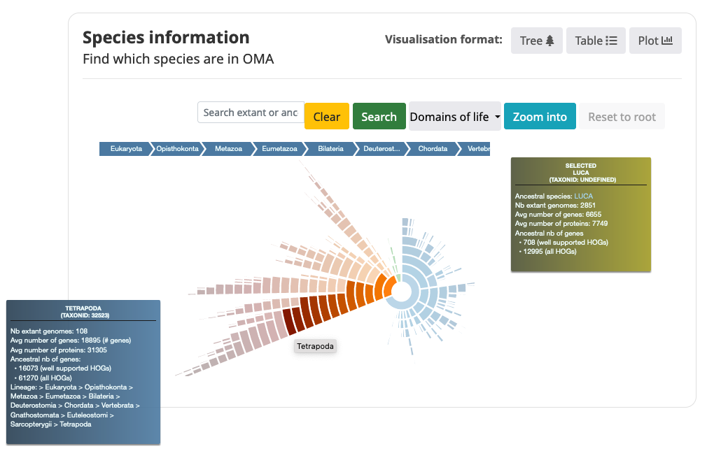
- Search for taxon (ancestral or extant species name) in the search bar.
- Mouse over the sections in the Taxon Hierarchy View to get information about the genome content.
- Name of taxon
- NCBI Taxon identifier
- Number of extant genomes in this clade
- Average number of genes for the extant species in this clade (Only includes 1 representative isoform per locus)
- Average number of proteins for the extant species in this clade (may include multiple isoforms)
- Number of ancestral genes for this clade, including all HOGs and well-supported HOGs (with a Completeness Score >= 0.3)
- Taxonomic lineage
- Change color of the Taxon Hierarchy View to color clades by clicking on the drop-down menu.
- By default the sunburst is colored by Domains of life (Eukaryota, Bacteria, Archaea)
- You can also color the sunburst by the average number of proteins/genes, or number of HOGs/well-supported HOGs.
- Zoom into a taxon by clicking on it in the sunburst or searching for it and clicking the “Zoom into” button.
Species Table View
The default view is the Taxon Hierarchy view. Each section in the Taxon Hierarchy View represents a clade or species at the tips of the viewer.
- Columns displayed:
- Code: 5-letter UniProt species code
- Scientific Name
- Common Name
- Last Update: When the genome was last updated in OMA
- # of Genes: the number of genes in this genome
- # of Sequences: includes all the alternative splice variants that are included in OMA
- Taxon Id: NCBI / GTDB taxon identifier. Negative numbers indicate GTDB assembly accessions
- D.: Domain of life (Bacteria, Archaea, Eukaryota)
- Search the table for species with the search bar above the table
- Display certain columns of the table with the filter icon in the top right
- Download the data by the download icon
Species Plot
View the number of genes per species plotted in a bar graph. The different Archaea, Bacteria, and Eukaryota domains are colored blue, green, and red, respectively.
- Sort bars by number of genes (size), Kingdom (domain), or Species Name (alphabetical order)
- Select which domain to show.
- View in either a compacted view or expanded view where it's possible to see every species’ name.
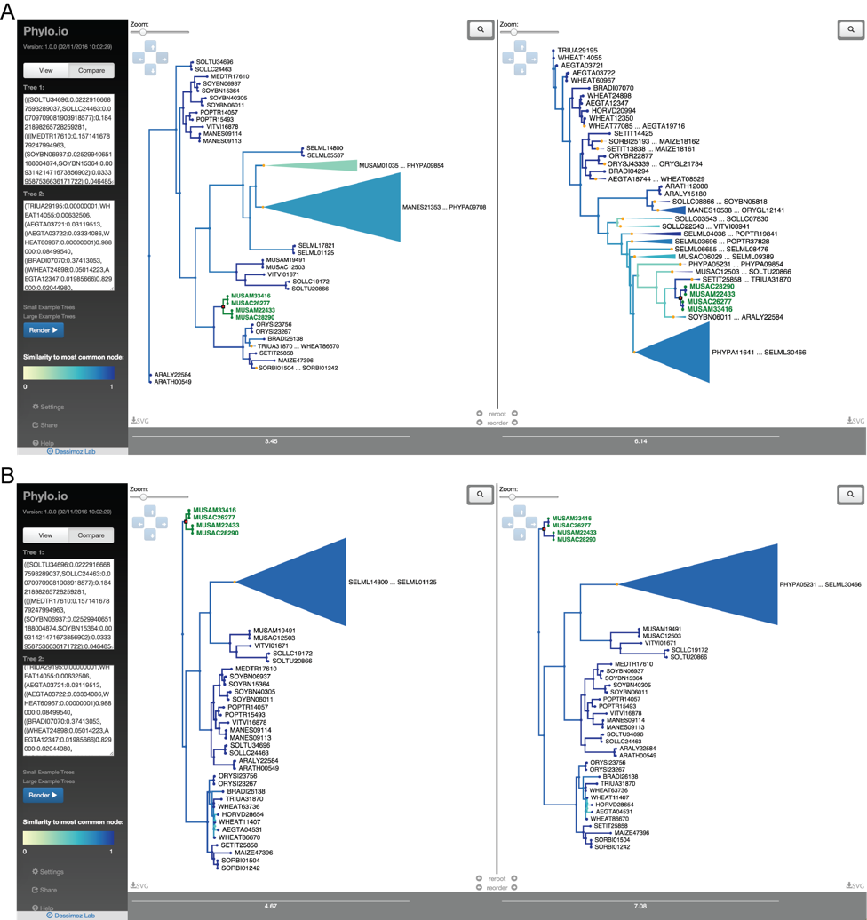
Phylo.io
Phylogenetic trees are pervasively used to depict evolutionary relationships. Increasingly, researchers need to visualize large trees and compare multiple large trees inferred for the same set of taxa (reflecting uncertainty in the tree inference or genuine discordance among the loci analyzed). Existing tree visualization tools are however not well suited to these tasks. In particular, side-by-side comparison of trees can prove challenging beyond a few dozen taxa.
Phylo.io is a web application to visualize and compare phylogenetic trees side-by-side.
Its distinctive features are:
- highlighting of similarities and differences between two trees
- automatic identification of the best matching rooting and leaf order
- scalability to large trees
- high usability
- multiplatform support via standard HTML5 implementation
- Possibility to store and share visualizations
The tool can be freely accessed at http://phylo.io and can easily be embedded in other web servers.
For more information:
- Paper: (Robinson et al. 2016)
- Github: The code for the associated JavaScript library is available at https://github.com/DessimozLab/phylo-io under an MIT open source license.
- Manual: http://phylo.io/manual.html
- Blog post: https://lab.dessimoz.org/blog/2016/04/28/phylo-io-software-to-visualise-and-compare-phylogenetic-trees
- Youtube video: https://www.youtube.com/watch?v=IOQK3CP8GlA&feature=emb_logo